2019-10-15 •

The adjoint method and its application in back-propagation of dominant eigen-decomposition

The adjoint method provides a new way of thinking about and deriving formulas for certain computation process. In this article, we will present the basic ideas of the adjoint method and, as a concrete example, demonstrate its consequences in back-propagation of the dominant eigen-decomposition and its relation with the traditional approach.

$\renewcommand{\vec}[1]{\mathbf{#1}}$

Basic ideas of the adjoint method

Consider a simple computation process, in which the setting is as follows. Let $\vec{p} = (p_1,\cdots, p_P)$ be a $P$-dimensional input vector of parameters, and the output $\vec{x} = (x_1, \cdots, x_M)^T$ is a $M$-dimensional (column) vector. They are related by $M$ equations of the form $f_i(\vec{x}, \vec{p}) = 0$, where $i$ ranges from $1$ to $M$.

What we need is the back-propagation of this process, in which the adjoint $\overline{\vec{p}} \equiv \frac{\partial \mathcal{L}}{\partial \vec{p}}$ of input is expressed as a function of the adjoint $\overline{\vec{x}} \equiv \frac{\partial \mathcal{L}}{\partial \vec{x}}$ of output. We have

$\overline{p_\mu} = \overline{\vec{x}}^T \frac{\partial \vec{x}}{\partial p_\mu}, \quad \forall \mu = 1, \cdots, P. \label{eq: adjointp}$

where the $M$-dimensional column vector $\frac{\partial \vec{x}}{\partial p_\mu}$ is determined by

$\frac{\partial f_i}{\partial p_\mu} + \frac{\partial f_i}{\partial \vec{x}} \frac{\partial \vec{x}}{\partial p_\mu} = 0, \quad \forall i = 1, \cdots, M.$

Or, we can express this in a more compact form as follows:

$\frac{\partial f}{\partial p_\mu} + \frac{\partial f}{\partial \vec{x}} \frac{\partial \vec{x}}{\partial p_\mu} = 0. \label{eq: partialxpartialp}$

where

$\frac{\partial f}{\partial p_\mu} = \begin{pmatrix} \frac{\partial f_1}{\partial p_\mu} \\ \vdots \\ \frac{\partial f_M}{\partial p_\mu} \end{pmatrix}, \quad \frac{\partial f}{\partial \vec{x}} = \begin{pmatrix} \text{—} & \frac{\partial f_1}{\partial \vec{x}} & \text{—} \\ & \vdots \\ \text{—} & \frac{\partial f_M}{\partial \vec{x}} & \text{—} \end{pmatrix}$

Assuming the $M \times M$ matrix $\frac{\partial f}{\partial \vec{x}}$ is invertible, one can solve for $\frac{\partial \vec{x}}{\partial p_\mu}$ from Eq. $\eqref{eq: partialxpartialp}$, then substitute it back into Eq. $\eqref{eq: adjointp}$ to get the final result:

$\begin{align} \overline{p_\mu} &= -\overline{\vec{x}}^T \left( \frac{\partial f}{\partial \vec{x}} \right)^{-1} \frac{\partial f}{\partial p_\mu} \\ &= -\boldsymbol{\lambda}^T \frac{\partial f}{\partial p_\mu}. \quad \forall \mu = 1, \cdots, P. \label{eq: adjointp in general case} \end{align}$

where the column vector $\boldsymbol{\lambda}$ is determined by

$\left( \frac{\partial f}{\partial \vec{x}} \right)^T \boldsymbol{\lambda} = \overline{\vec{x}}. \label{eq: lambda in general case}$

Example: dominant eigen-decomposition

As a concrete example of the adjoint method, consider the dominant eigen-decomposition process, in which a certain eigenvalue $\alpha$ and corresponding eigenvector $\vec{x}$ of $A$ is returned (assuming the eigenvalue is non-degenerate), where $A = A(\vec{p})$ is a $N \times N$ real symmetric matrix depending on the parameter $\vec{p}$.

Note that in the current case, the output can be effectively treated as a vector of dimension $N + 1$. The correspondence with the general notations in the last section is thus as follows:

$\vec{x} \rightarrow \begin{pmatrix} \vec{x} \\ \alpha \end{pmatrix}, \quad \overline{\vec{x}} \rightarrow \begin{pmatrix} \overline{\vec{x}} \\ \overline{\alpha} \end{pmatrix}, \quad \boldsymbol{\lambda} \rightarrow \begin{pmatrix} \boldsymbol{\lambda} \\ k \end{pmatrix}, \quad \frac{\partial f}{\partial p_\mu} \rightarrow \begin{pmatrix} \frac{\partial f_1}{\partial p_\mu} \\ \vdots \\ \frac{\partial f_N}{\partial p_\mu} \\ \frac{\partial f_0}{\partial p_\mu} \end{pmatrix}, \\ \left( \frac{\partial f}{\partial \vec{x}} \right)^T = \begin{pmatrix} \vert & & \vert \\ \left( \frac{\partial f_1}{\partial \vec{x}} \right)^T & \cdots & \left( \frac{\partial f_M}{\partial \vec{x}} \right)^T \\ \vert & & \vert \end{pmatrix} \rightarrow \left(\begin{array}{ccc|c} \vert & & \vert & \vert \\ \left( \frac{\partial f_1}{\partial \vec{x}} \right)^T & \cdots & \left( \frac{\partial f_N}{\partial \vec{x}} \right)^T & \left( \frac{\partial f_0}{\partial \vec{x}} \right)^T \\ \vert & & \vert & \vert \\ \hline \frac{\partial f_1}{\partial \alpha} & \cdots & \frac{\partial f_N}{\partial \alpha} & \frac{\partial f_0}{\partial \alpha} \end{array}\right).$

The $N + 1$ equations $f_i(\vec{x}, \alpha, \vec{p}) = 0$ are given by

$f_i(\vec{x}, \alpha, \vec{p}) = (A - \alpha I)_i^T \vec{x}, \quad \forall i = 1, \cdots, N. \\ f_0(\vec{x}, \alpha, \vec{p}) = \vec{x}^T \vec{x} - 1. \label{eq: fs}$

where the subscript $i$ denotes the $i$th column of the matrix $A - \alpha I$, and the extra equation $f_0(\vec{x}, \alpha, \vec{p}) = 0$ imposes the normalization constraint. Using Eq. $\eqref{eq: fs}$, one can easily obtain that

$\left( \frac{\partial f}{\partial \vec{x}} \right)^T \rightarrow \begin{pmatrix} A - \alpha I & 2\vec{x} \\ -\vec{x}^T & 0 \end{pmatrix}.$

In correspondence with Eq. $\eqref{eq: lambda in general case}$ in the general case, the matrix equation satisfied by $\boldsymbol{\lambda}$ and $k$ thus yields

$(A - \alpha I) \boldsymbol{\lambda} + 2k\vec{x} = \overline{\vec{x}}. \\ -\vec{x}^T \boldsymbol{\lambda} = \overline{\alpha}. \label{eq: matrix equation of lambda and k}$

One can solve for $k$ by multiplying both sides of the first equation by $\vec{x}^T$, and obtain

$2k = \vec{x}^T \overline{\vec{x}}.$

Substituting it back to Eq. $\eqref{eq: matrix equation of lambda and k}$, one can obtain the unique solution for $\boldsymbol{\lambda}$ as follows:

$\boldsymbol{\lambda} = -\overline{\alpha} \vec{x} + \boldsymbol{\lambda}_0, \quad \textrm{where $\boldsymbol{\lambda}_0$ satisfies} \\ \color{red}{ (A - \alpha I)\boldsymbol{\lambda}_0 = (1 - \vec{x}\vec{x}^T) \overline{\vec{x}}, \quad \vec{x}^T \boldsymbol{\lambda}_0 = 0. } \label{lambda0}$

The vector $\boldsymbol{\lambda}_0$ in the equation above can be solved by Conjugate Gradient (CG) method.

Finally, note that in the current case,

$\frac{\partial f}{\partial p_\mu} \rightarrow \begin{pmatrix} \frac{\partial A}{\partial p_\mu} \vec{x} \\ 0 \end{pmatrix}$

In correspondence with Eq. $\eqref{eq: adjointp in general case}$, one thus obtains

$\begin{align} \overline{p_\mu} &= -\boldsymbol{\lambda}^T \frac{\partial A}{\partial p_\mu} \vec{x} \\ &= (\overline{\alpha} \vec{x}^T - \boldsymbol{\lambda}_0^T) \frac{\partial A}{\partial p_\mu} \vec{x}. \end{align}$

Or, one can “strip” the parameter $\vec{p}$ out of the function primitive and obtain the expression of $\overline{A}$ by taking account of the fact that $\overline{p_\mu} = \textrm{Tr}\left(\overline{A}^T \frac{\partial A}{\partial p_\mu}\right)$. The final result is

$\color{red}{ \overline{A} = (\overline{\alpha} \vec{x} - \boldsymbol{\lambda}_0) \vec{x}^T. } \label{result: dominant diagonalization}$

Fairly simple.

Relation with the derivation based on full eigen-decomposition

Now, let’s try to figure out the relation of the above approach based on adjoint method with that of the full eigen-decomposition process. The only difference is that compared with the full diagonalization formulation, the adjoint method presented above only needs one specific eigenvalue(usually the smallest or the largest one) and corresponding eigenvectors. Nevertheless, we can “wrap” the process of full diagonalization within the dominant eigen-decomposition and utilize the results of the former formulation in the latter, as demonstrated in the figure below.

2019-10-14-full_diagonalization

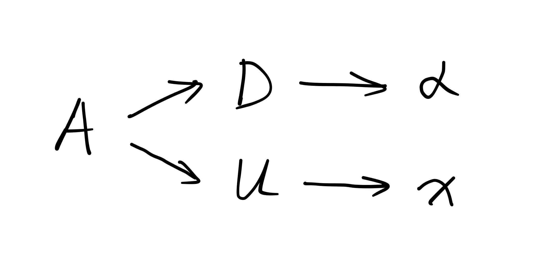
For clarity and without loss of generality, let $\alpha$ and $\vec{x}$ be the “first” eigenvalue and corresponding eigenvector of the matrix $A$. That is, we have $U^T A U = D$, where

$D = \begin{pmatrix} \alpha \\ & \alpha_2 \\ & & \ddots \\ & & & \alpha_N \end{pmatrix}, \quad U = \begin{pmatrix} \vert & \vert & & \vert \\ \vec{x} & \vec{x}_2 & \cdots & \vec{x}_N \\ \vert & \vert & & \vert \end{pmatrix}$

Recall that the full eigen-decomposition gives the following backward formula of $\overline{A}$ in terms of $\overline{D}$ and $\overline{U}$:

$\overline{A} = U (\overline{D} \circ I + U^T \overline{U} \circ F) U^T. \label{eq: full diagonalization AD}$

where $F$ is an anti-symmetric matrix with off-diagonal elements $F_{ij} = (\alpha_j - \alpha_i)^{-1}$. For more details, see the references in the last section. On the other hand, the dominant eigen-decomposition described above yields the following relations between $\overline{D}, \overline{U}$ and $\overline{\alpha}, \overline{\vec{x}}$:

$\overline{D} \circ I = \begin{pmatrix} \overline{\alpha} \\ & 0 \\ & & \ddots \\ & & & 0 \end{pmatrix}, \quad \overline{U} = \begin{pmatrix} \begin{array}{c|} \vert \\ \overline{\vec{x}} \\ \vert \end{array} & \begin{array}{ccc} \\ & \Huge{0} & \\ & \end{array} \end{pmatrix}.$

Then one can obtain through simple algebraic manipulation that

$\overline{D} \circ I + U^T \overline{U} \circ F = \begin{pmatrix} \begin{array}{c|} \overline{\alpha} \\ \frac{1}{\alpha - \alpha_2} \vec{x}_2^T \overline{\vec{x}} \\ \vdots \\ \frac{1}{\alpha - \alpha_N} \vec{x}_N^T \overline{\vec{x}} \end{array} & \begin{array}{ccc} \\ & \Huge{0} & \\ & \end{array} \end{pmatrix} \equiv \begin{pmatrix} \begin{array}{c|} \overline{\alpha} \\ -c_2 \\ \vdots \\ -c_N \end{array} & \begin{array}{ccc} \\ & \Huge{0} & \\ & \end{array} \end{pmatrix}.$

where we have introduced the quantities $c_i = \frac{1}{\alpha_i - \alpha} \vec{x}_i^T \overline{\vec{x}}, \quad \forall i = 2, \cdots, N$. Substituting this equation back into $\eqref{eq: full diagonalization AD}$, we have

$\overline{A} = \overline{\alpha} \vec{x} \vec{x}^T - \sum_{i=2}^N c_i \vec{x}_i \vec{x}^T. \label{result: full diagonalization}$

This formula looks very similar to the result $\eqref{result: dominant diagonalization}$ obtained from the adjoint method. Actually they are identically the same. This can be seen by expanding the vector $\boldsymbol{\lambda}_0$ characterized in Eq. $\eqref{lambda0}$ in the complete basis $(\vec{x}, \vec{x}_2, \cdots, \vec{x}_N)$. One can easily see that the quantities $c_i$ defined above are exactly the linear combination coefficients of $\boldsymbol{\lambda}_0$ in this basis. In other words, we have

$\boldsymbol{\lambda}_0 = \sum_{i=2}^N c_i \vec{x}_i.$

Plugging this result back into $\eqref{result: full diagonalization}$ clearly reproduces the earlier result $\eqref{result: dominant diagonalization}$.

Remarks

The observation above clarifies the equivalence of the two formulations of deriving the back-propagation of the dominant eigen-decomposition process. The fact that the final result is identically the same is not surprising, but the “native” representations of the result are indeed different from a practical point of view. In the formulation based on adjoint method, one only makes use of the “dominant” eigenvalue and eigenvector instead of the full spectrum, thus allowing for the construction of a valid dominant eigensolver function primitive in the framework of automatic differentiation. In a typical implementation, the forward pass can be accomplished by Lanczos or other dominant diagonalization algorithms, while the backward pass can be implemented by solving the linear system $\eqref{lambda0}$ using Conjugate Gradient method. In the case of large matrix dimension, this approach is clearly more efficient.

References

The presentation of general ideas of adjoint method and its application in dominant eigen-decomposition is largely based on this notes:

https://math.mit.edu/~stevenj/18.336/adjoint.pdf

There are some good notes on automatic differentiation of basic matrix operations, including the full eigen-decomposition process. For example:

https://people.maths.ox.ac.uk/gilesm/files/NA-08-01.pdf